

Introduction
Welcome back to our blog series covering the fundamentals of biosignals processing. In our first blog post of this series, we set the stage for biosignals and biosignals processing, what it is, and where you can encounter real-world applications.
We’ve already identified that biosignals are a crucial source of information from which we can extract parameters and features that allow us to understand the human body better and make decisions on its state and health. For instance, an athlete might want to understand better how their body reacts to their training, find possible injury risks, and build upon what works best to improve their performance.
To ensure that we are making the right decisions we have to ensure that we are looking at noise-free biosignals, otherwise noise might lead us to the wrong conclusions. For instance, a signal impacted by motion artifacts, if left untreated, may convince us falsely that the signal distortion is of pathological nature. But before we proceed with removing components from our signals, we need to better understand what we actually need or want to remove.
In this second post, we will have a look at different examples of noise sources, signal artifacts, and other types of interferences we may encounter when working with raw, unfiltered biosignals. We’ll also learn about a useful tool, the Signal-to-Noise Ratio, that helps quantify the quality of our signal.
Understanding Artifacts & Noise Sources
A conflict of biosignals
Measuring biosignals is often easier than expected as we can extract a variety of them directly on the skin surface. However, there’s a lot going on underneath the skin that can cause interference, such as different organs overlapping each other resulting in overlapped biosignals.
For instance, when measuring an Electrocardiography (ECG) sensor by placing the sensors on the chest’s skin surface, there is still a chest muscle between the electrode and the heart from which we want to get the actual ‘true’ biosignal from. From a physiological point of view, the chest muscle and the heart may be made out of muscles but they have significant differences. You can control the former but can’t control the latter among other differences. Fortunately, you don’t have to think about your every heartbeat as if you’d be flexing your biceps - your heart handles this itself!
However, from an electrical point of view, the biosignals of the heart and the skeletal muscles have characteristics that overlap, such as their amplitudes ranging from -1.5mV to 1.5mV or frequencies ranging from 0.05Hz to 100Hz (and beyond). It’s for this reason that you may encounter interferences in raw ECG data during the activity of the chest muscle. Here, when using an ECG sensor to collect raw ECG data, the activity of the muscles between the electrode and the heart can interfere with the ECG signal.
We can experience this as heavy distortions of the ECG signal (e.g. rapid arm movement) or slow changes in the ECG baseline over time (baseline wandering) that can be caused by the respiration movements among other factors.
Motion Artifacts
Movement, both voluntary and involuntary, is unavoidable in most research setups. After all, there would be little biosignals to record if a research participant would not be allowed to breathe through an entire data recording.
Movement can significantly impact biosignals recordings either through the interference of biosignals that are responsible for the movement, such as muscle activity or for mechanical reasons, as movement can impact the contact between the sensor and the skin surface.
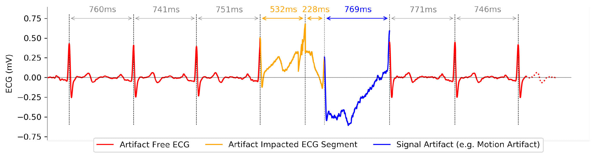
The following example shows a typical impact of movement on a raw ECG recording. Here, the baseline is significantly shifted during the signal segment and the distortion can even lead to additional peaks in the signal that may be misinterpreted as R-peaks, which act as heartbeat indicators in the ECG signal.
The challenge: Getting the motion artifact impacted ECG signal from this…
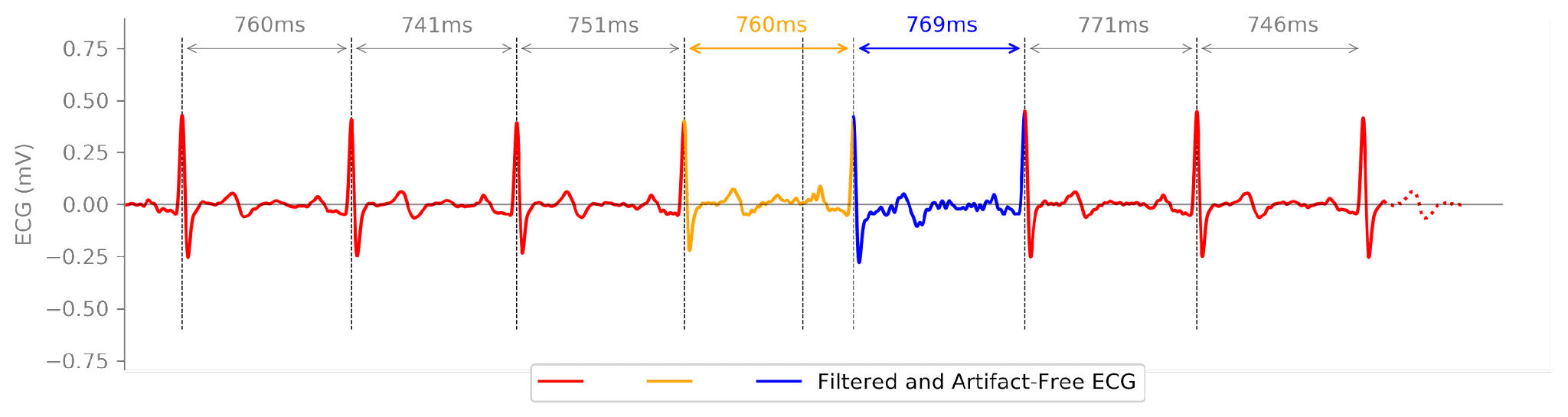
…back to its original form like this:
Powerline Noise (50Hz / 60Hz)
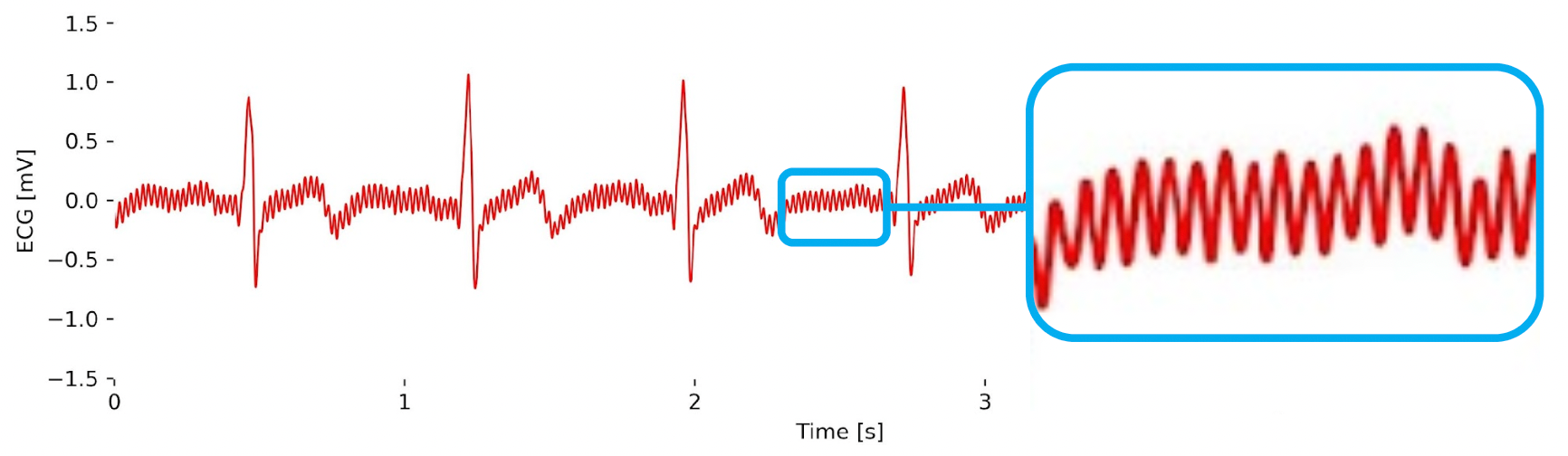
Depending on where you are in the world, the power in your house, office, or lab may be provided as a 50Hz (e.g. EU) or 60Hz (e.g. USA) alternate signal. This continuous cycling creates a rhythmic electromagnetic field around powerlines and electrical equipment that may be captured by your biosignals sensors. This type of noise can sneak in through a variety of different ways into your biosignals, even if your sensor provides a shielded cable. For instance, an electrode with a big enough metallic electrode-sensor connector can capture noise like this:
Fortunately, you don’t have to unplug everything around you and record good biosignals data in the dark, especially because you cannot always even fully control your environment.
Measuring Signal Quality: Signal-to-Noise Ratio
Before we head straight into the tools that help us remove noises from our biosignals, we need to ask ourselves first how badly our biosignals are impacted by the available noise. Understanding the quality of your biosignals is vital to select the best pre-processing steps.
One crucial metric that guides us in this quest is the Signal-to-Noise Ratio (SNR) which we’ll cover further with an interactive Python notebook below.
What is the Signal-to-Noise Ratio (SNR)?
Imagine you're in a bustling room, trying to have a conversation with someone amidst background chatter and noise. The challenge lies in distinguishing the person's voice (the signal) from the surrounding distractions (the noise).
As we’ve seen in the previous examples, in biosignal processing, we encounter a similar situation: the signal represents the physiological information we want to study (e.g. ECG), while the noise comprises various interferences and unwanted elements that obscure the signal (e.g. power line noise).
The Signal-to-Noise Ratio (SNR) is a quantitative measure that assesses the clarity of the signal present in the biosignal data. It compares the strength of the actual signal to the level of unwanted noise present in the recording. A higher SNR indicates a clearer and more distinct signal, making it easier to analyze and draw meaningful conclusions, while a lower SNR suggests a weaker signal partially buried in noise.
Computing the Signal-to-Noise Ratio (SNR)
Computing the Signal-to-Noise Ratio (SNR) involves a straightforward yet essential mathematical process. To determine the SNR of a biosignal, we first calculate the mean amplitude of the signal, representing the genuine physiological information we want to extract (e.g. EEG waveform). Next, we measure the standard deviation of the noise present in the signal (e.g. baseline noise), representing the unwanted interferences and background disturbances. Dividing the mean signal amplitude by the standard deviation of the noise results in the SNR value, which quantifies the strength of the signal relative to the level of interference.
For a hands-on understanding, we have prepared a biosignals notebook with practical examples showcasing how to compute the SNR using an EEG sensor signal. This notebook guides you through step-by-step implementations, enabling you to grasp the concept and apply it to your own biosignal processing endeavors.
📙 Python Notebook: Computing the Signal-to-Noise Ratio
Coming Up! Pre-processing Methods: Removing noise from raw biosignals
In this blog post, we learned various examples of noise sources and how they impact our biosignals. In addition, we also learned a valuable tool to quantify how noisy our signal is, the Signal-to-Noise Ratio (SNR).
In the next post, we’ll cover fundamental pre-processing methods that aim to remove noise and unwanted interferences from our biosignals to ensure that we are extracting features from clean data and avoiding mistakenly identifying noise sources as potential abnormal physiological conditions.